About

The server has two principal functions.

First, it processes the stack of user-supplied 1D PFG NMR spectra and integrates the signal over a specified spectral region. In doing so, the algorithm determines a shape of the spectrum in the region of interest,

$f_{model} (\omega)$ , and then fits the individual spectra using this model. This step maximizes S/N ratio of the integrated data,

$I(g_k )$ (see below for further details).

Second, the integrals

$I(g_k )$ are fitted using Stejskal-Tanner or Jerschow and Müller equation as appropriate. The data are plotted along with the best-fit curve and the fitted diffusion coefficient is reported.

Integration algorithm

(i) Linear baseline correction is applied to all spectra

$f_k (\omega)$ using left and right endpoints of the region of interest,

$\omega_{left}$ and

$\omega_{right}$ .

(ii) The obtained spectra are integrated over the interval from

$\omega_{left}$ to

$\omega_{right}$ . The resulting integrals

$s_k$ suffer from noise, which arises, inter alia , from the use of 2-point baseline correction in the previous step.

(iii) A model spectrum is obtained by calculating the weighted average of all spectra. The weights are set to

$s_k$ , as evaluated in the previous step:

$f_{model} (\omega)=\dfrac{ \sum_{k=1}^{N} s_k f_k (\omega) }{ \sum_{k=1}^{N} s_k }$
The weighting scheme is based on the idea of matched filtering, which maximizes the signal-to-noise ratio of the resultant model spectrum [R. R. Ernst, G. Bodenhausen, A. Wokaun, Principles of nuclear magnetic resonance in one and two dimensions, Oxford University Press, Oxford, 1987; R. G. Spencer, Concepts Magn. Reson. A 2010, 36, 255].

(iv) All spectra

$f_k (\omega)$ are approximated using the ansatz

$a_k+b_k \omega+c_k f_{model} (\omega)$ . The term

$a_k+b_k \omega$ is intended to refine the baseline correction performed in step (i). The term

$c_k f_{model} (\omega)$ represents the spectrum per se, assuming that each spectrum

$f_k (\omega)$ can be expressed as a scaled version of the model spectrum. The constants

$a_k$ ,

$b_k$ , and

$c_k$ are fitted by minimizing the following target function:

$\int_{\omega_{left}}^{\omega_{right}} \Big(( a_k+b_k \omega+c_k f_{model} (\omega) ) - f_k (\omega) \Big)^2 d\omega$
The coefficients

$c_k$ are taken to be the experimental values of

$I(g_k )$ . A detailed characterization of this scheme, including its superior properties with respect to noise suppression, will be published in the Journal of Biomolecular NMR.

Instructions

1) Process FIDs in TopSpin Software (ft, phase and baseline correction).
2) Choose the appropriate integration region (you can select the boundaries in ppm or in points). The region must contain spectral signals from only one type of molecular species (or otherwise different species with identical diffusion properties). As always, stay away from the residual solvent signal. For best performance choose an isolated region, where the left and right boundaries are at or near the baseline (e.g. methyl region).
3) Choose the desired protocol at the DDfit homepage (either an appropriate pulse sequence or data integration only).
4) Select all appropriate spectrometer files (2rr, procs, proc2s, difflist).
5) Fill in the requested experimental parameters (briefly summarized below).
4) Input all required experiment parameters (see description below) depended on the experiment type.
6) Click submit button. The computations take a few seconds.
7) Inspect the results page (which is assigned a unique URL).

You can see demo page for live demonstration.

Experiment types

Stimulated Echo experiment

Pulse sequence:

Stejskal-Tanner equation (link):

$I(g) = exp\Bigg(-D\gamma ^{2}g^{2}\delta ^{2}\left(\Delta -\dfrac{\delta}{3}\right)\Bigg)$

using Bruker notations (Bruker program stegp3s):

$I(g) = exp\Bigg(-D\gamma^{2}g^{2} {(p30)}^{2}\left(d20 -\dfrac{p30}{3}\right)\Bigg)$

Experiment parameters:

Gyromagnetic ratio: 𝛄
Gradient strength: g
Gradient length: 𝛅 = p30
Diffusion delay: 𝚫 = d20
Diffusion coefficient: D

Stimulated Echo experiment using bipolar gradients

Pulse sequence:

Stejskal-Tanner equation modified by Jerschow and Müller (link):

$I(g) = exp \Bigg(-D\gamma ^{2}g^{2}\delta ^{2}\left(T + \dfrac{2}{3}\delta + \dfrac{3}{4}\tau \right)\Bigg)$

using Bruker notations (Bruker program stegpbp3s):

$I(g) = exp \Bigg(-D\gamma ^{2}g^{2} {(2p30)} ^{2}\left(d20 - \dfrac{2}{3} p30 - \dfrac{d16}{2} - 4p1 \right)\Bigg)$

Experiment parameters:

Gyromagnetic ratio: 𝛄
Gradient strength: g
Gradient length: 𝛅 = 2p30
Diffusion delay: d20
Diffusion coefficient: D
Recovery delay: 𝛕 = 2d16
T = d20 - 2p30 - 2d16 - 4p1
p1 is 90° pulse duration

Double-Stimulated Echo Experiment

Pulse sequence:

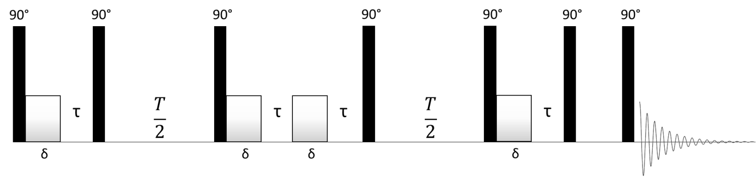
Stejskal-Tanner equation modified by Jerschow and Müller (link):

$I(g) = exp \Bigg(-D\gamma ^{2}g^{2}\delta ^{2}\left(T + \dfrac{4}{3}\delta + 2\tau \right)\Bigg)$

using Bruker notations (Bruker program dstegp3s):

$I(g) = exp \Bigg(-D\gamma ^{2}g^{2} {(p30)} ^{2}\left(d20 - \dfrac{5}{3} p30 - d16 - 4p1 \right)\Bigg)$

Experiment parameters:

Gyromagnetic ratio: 𝛄
Gradient strength: g
Gradient length: 𝛅 = p30
Diffusion delay: d20
Diffusion coefficient: D
Recovery delay: 𝛕 = d16
T = d20 - 3p30 - 3d16 - 4p1
p1 is 90° pulse duration

Double-Stimulated Echo Experiment using bipolar gradients

Pulse sequence:

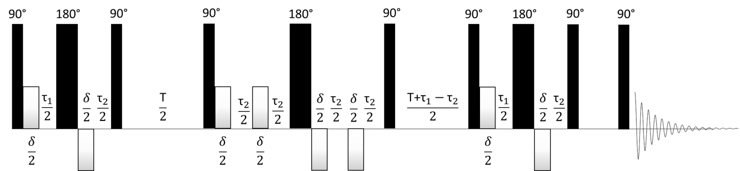
Stejskal-Tanner equation modified by Jerschow and Müller (link):

$I(g) = exp \Bigg(-D\gamma ^{2}g^{2}\delta ^{2}\left(T + \dfrac{4}{3}\delta + \dfrac{5}{4}\tau_1 + \dfrac{\tau_2}{4} \right)\Bigg)$

using Bruker notations (Bruker program dstebpgp3s):

$I(g) = exp \Bigg(-D\gamma ^{2}g^{2} {(2p30)} ^{2}\left(d20 - \dfrac{10}{3} p30 - 3d16 - 8p1 \right)\Bigg)$

Experiment parameters:

Gyromagnetic ratio: 𝛄
Gradient strength: g
Gradient length: 𝛅 = 2p30
Diffusion delay: d20
Diffusion coefficient: D
Recovery delay: 𝛕₁= 𝛕₂= 2d16
T = d20 - 6p30 - 6d16 - 8p1
p1 is 90° pulse duration